HOW TO USE

1. Dataset

An example dataset can be downloaded here.

2. DiagnoMass Setup

The latest version of the DiagnoMass software is available here. The software requires version 6.0.13 or higher of the .NET Desktop Runtime, which can be downloaded here if not installed.

3. Data Structure

3.1. Follow the data structure in folders (Figure 1)

Warning: Visualizing the spectra in item 6.2.1 is necessary to use this data structure. The raw files are deposited in PRIDE(PXD035961).

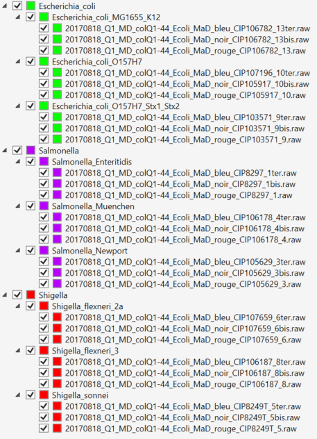
Figure 1.

4. Login (Figure 2)

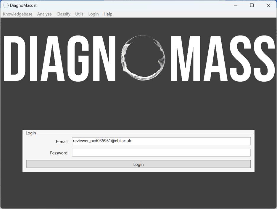
Figure 2.

4.1. Click on Login -> Register New User (Figure 3)

Figure 3. DiagnoMass is required to use a login and password. An existing user creates the login, allowing to identify the spread of software use.

5. Knowledgebase

5.1. Click on Knowledgebase -> Create Knowledgebase (Figure 4)

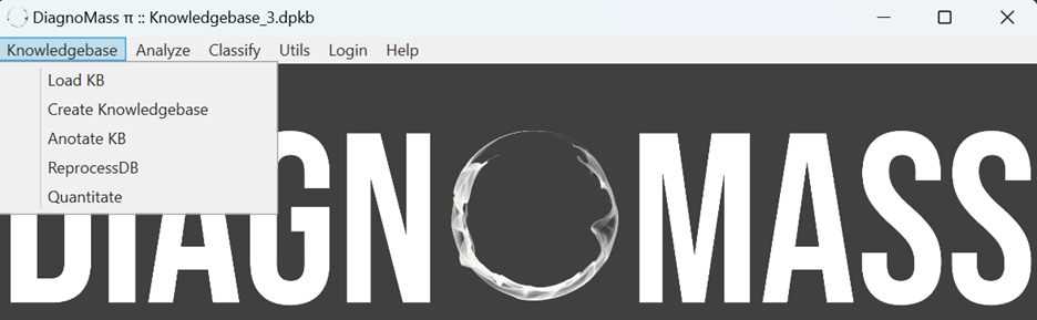
Figure 4.

5.2. Click on Add Directory (Figure 5)

5.3. Click on Generate (Figure 5)

Figure 5.

5.5.  Click on Knowledgebase -> Load KB (Figure 6)

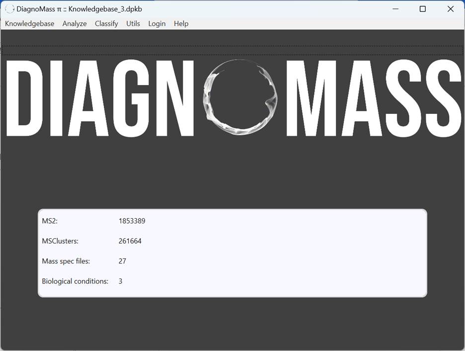
Figure 6.

5.4.  Click on knowledgebase -> Annotate KB (Figure 7)

Warning: The identification files must be inside the directories.

Figure 7.

6. Analyze

6.1. Click on Analyze -> Dimensional Reduction (Figure 8)

Figure 8. The dimensionality reduction viewer. The tree view shows the hierarchy of biological conditions, biological replicates, and technical replicates. Data visualization can provide plots generated with PCA or t-SNE.

6.2. Click on Analyze -> Heatmap (Figure 9)

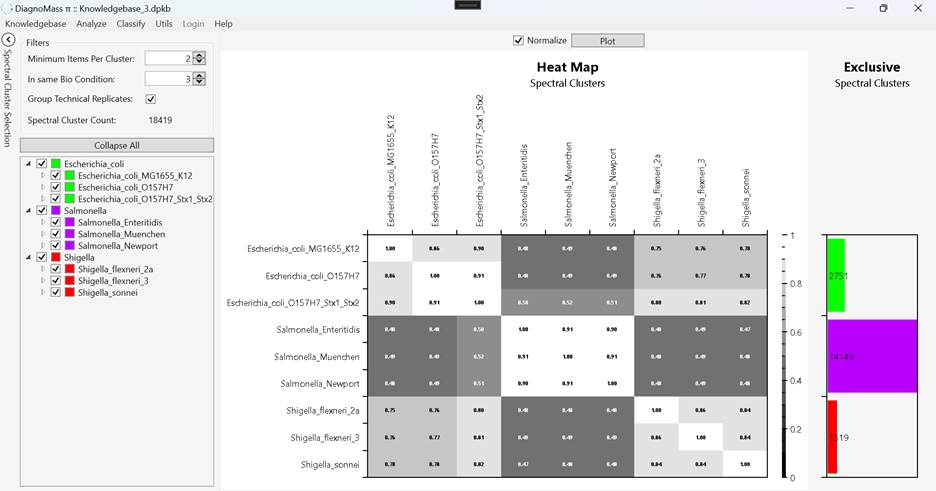
Figure 9. The comparison of all biological replicates generates a heat map; lighter shades denote more similar samples. On the right is a bar plot showing the number of exclusive spectral clusters for each condition. The discriminant cluster explorer (Supplementary figures 3 to 5) can be opened to explore the discriminant clusters by double-clicking on the respective column.

6.2.1. Click on Analyze -> Heatmap -> Exclusive Spectral Clusters (Figure 10)

Figure 10. A screenshot of the DiagnoMass discriminant cluster explorer. The Spectral Clusters Identified group box reports the number of clusters annotated and the total number of spectral clusters for a given condition. Inside this group box is a table reporting the discriminant cluster IDs, and for each cluster, the number of spectra (#MS2), the number of protein Loci (#Sequences) as per the PLV peptide identifications, Purity (i.e., a cluster with all spectra identified as the same peptide will have a purity of 100%; if there are no identifications the purity will be -1), Purity Seq (i.e., a cluster having conflicting results reported from different search engines will not achieve 100% sequence purity), and Peptides (the sequence with the highest PLV identification score). The MS2 group box lists information on spectra belonging to the cluster selected in the Spectral Clusters Identified group box. This screenshot refers to a spectral cluster (Id = 120280, Precursor m/z = 1421.1687, z=2) found only in E. coli and unidentified by PLV, Novor, and FragPipe. The upper-right group box shows the Consensus Spectrum generated using all spectra belonging to the selected cluster. The lower-right group box, Experimental Spectrum, shows a spectrum belonging to the selected spectral cluster; in this case, the one highlighted in blue in the MS2 group box.

7. Classify

7.1. Click on Browse and select the raw file to classify (Figure 11). The score (Item 7.2) represents in percentage.

Figure 11.

7.2. Scoring function

Given a total of  biological conditions, consider a spectrum appearing in  conditions (i.e., ) and having cosine score  relative to a given reference spectrum. The scoring function we use for the new spectrum given this reference is , where  is the well-known logistic function, in this case, centered at . That is:

In this expression,  controls the slope of the curve and is chosen so that, given a value for parameter , we have  and . This criterion yields

For a negative slope, we need . An illustration is given in supplementary figure 12.

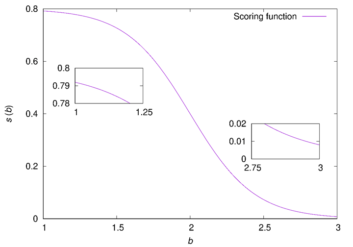
Figure 12. Plot of  for , , and . The two insets zoom in on the extrema of , highlighting  and .